
You define a sequence of abelian groups A0, A1, A2,... connected by homomorphisms
dn : An → An - 1
such that the composition of any two consecutive maps is zero

dn o dn + 1 = 0
for all n. This sequence is called a chain complex. This means that the image of the (n + 1)-th map is contained in the kernel of the n-th map, and we can define the n-th homology group X to be the factor group
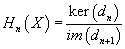
Hn(X) = ker(dn)/im(dn + 1)
A chain complex is called exact if the image of the (n + 1)-th map is always equal to the kernel of the n-th map. The homology groups of X therefore measure how far the chain complex associated to X is from being exact.
Let's say you have a simplicial complex X. Here An is the free abelian group whose generators are n-dimensional oriented simplices of X. The mappings are called the boundary mappings and send the simplices with vertices
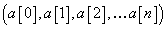
(a[0], a[1], a[2],...a[n])
to the sum
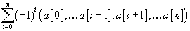
[summation of i from 0 to n ](-1)i (a[0], ...., a[i - 1], a[i + 1],...a[n])
If you take the modules to be over a field, then the dimension of the n-th homology of X turns out to be the number of holes in X at dimension n.
You can define a simplicial homology for any topological space X by defining a chain complex for X by taking An to be the free abelian group whose generators are all continuous maps from n-dimensional simplices into X. The homomorphisms dn arise from the boundary maps of the simplices.
A homology group is an abelian group that partially counts the holes in a topological space. Singular homology groups form a measure of the hole structure of a space, but they are one particular measure, and they don't always pick up everything.
The fundamental groups of a topological space X are related to its first singular homology group because a loop is also a singular 1-cycle. Mapping the homotopy class of each loop at its base point x0 to the homology class of the loop gives a homomorphism from the fundamental group π1(X, x0) to the homology group H1(X). If X is path-connected, then this homomorphism is surjective, and its kernel is the commutator subgroup of π1(X, x0), and H1(X) is therefore isomorphic to the abelianization of π1(X, x0).
The Betti numbers of a topological space X are an infinite sequence of numbers, b0, b1, b2,...,which are invariants of a topological space. Each Betti number is either a natural number, 0, 1, 2,..., or infinity. For most reasonable spaces, such as compact manifolds, finite simplicial complexes, or CW complexes, the sequence of Betti numbers, which consists of natural numbers, is zero from some point onwards, meaning all the Betti numbers after some point in the sequence are zero. The term "Betti numbers" was invented by Henri Poincare (1854 - 1912), and was named after Enrico Betti.
The k-th Betti number

bk(X)
of the space X is defined as the rank of the abelian group

Hk(X)
The k-th homology group of X.
You can also define it as a vector space dimension of

Hk(X, Q)
Since the homology group in this case is a vector space over Q. The universal coefficient theorem shows that these definitions are the same.
More generally, given a field F, you can define

bk(X, F)
the k-th Betti number with coefficient in F, as the vector space dimension of

Hk(X, F)
The Betti numbers bk(X) do not take into account any torsion in the homology groups, but they are still very useful. Basically, they allow you to count the number of holes of different dimensions. For a circle, the first Betti number is 1. For a general pretzel, the first Betti number is twice the number of holes. In the case of a finite simplicial complex, the homology groups Hk(X, Z) are finitely-generated, and so have a finite rank. The rank of the group is zero when k exceeds the dimension of a simplex of X.
For a finite CW-complex K, you have
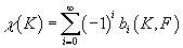
χ(K) = [summation over i from 0 to infinity] (-1)ibi(K, F)
where χ(K) is the Euler characteristic of K and any field F.
For any two spaces X and Y, you have

PX x Y = PXPY
Where PX is the Poincare polynomial of X, which is the generating function of the Betti numbers of X.

PX = b0(X) + b1(X)z + b2(X)z2 + ...
If X is an n-dimensional manifold, there is a symmetry interchanging k and n - k, for any k.
bk(X) = bn - k(X)
The dependence on the field F is only through its characteristic. If the homology groups are torsion-free, the Betti numbers are independent of F. The connection of p-torsion and the Betti number for a characteristic p, where p is a prime number, is given in detail by the universal coefficient theorem.
The Betti number sequence for a point, R0, is
1, 0, 0, 0,...
The Betti number sequence for a circle, S1, is
1, 1, 0, 0, 0,...
The Betti number sequence for a two-torus, T2, is
1, 2, 1, 0, 0, 0....
The Betti number sequence for a three-torus, T3, is
1, 3, 3, 1, 0, 0, 0,...
The Betti number sequence for a four-torus, T4 is
1, 4, 6, 4, 1, 0, 0, 0,...
Notice this reproduces Pascal's Triangle, invented by Blaise Pascal (1632 - 1662)
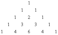
               1
            1	  1
        1     2     1
     1     3      3     1
1      4     6       4      1
where each number is the sum of the two numbers directly above it, with zeroes off the diagonal. The numbers in line n are the coefficients you get if you expand (x + y)n. Also, if you draw Pascal's Triangle, and color in the odd entries, you get a fractal called Sierpinski's Gasket.When Pascal wrote about Pascal's Triangle in 1654, he was merely rediscovering it. The basic idea of Pascal's triangle goes back to Mersenne in 1636, and Tartaglia in 1556, and the Hindu mathematician Bhaskara in 1150, and the Jain mathematician Mahavira in 850 A. D.
For any Rn, such as a point, line, plane, 3D space, 4D space, etc, or any subunit thereof, such as an interval, disk, ball, etc, the first Betti number is 1, and the rest are zero.
It's possible for spaces that are infinite-dimensional to have an infinite series of non-zero Betti numbers. An example is the infinite-dimensional complex projective plane, which has a sequence of 1, 0, 1, 0,.... which is periodic with period length 2. Here are examples of the Betti numbers of manifolds.
1. bn(S1) = 1, 1, 0, 0, 0,...
2. bn(T2) = 1, 2, 1, 0, 0, 0,...
3. bn(T3) = 1, 3, 3, 1, 0, 0, 0,...
4. bn(Rn) = 1, 0, 0, 0, 0,...
5. bn(CP∞) = 1, 0, 1, 0, 1, 0,...
Also, Betti numbers predict the dimensions of vector spaces of closed differential forms. The connection with the definition given above is from three different results, which are de Rham's theorem, Poincare’s duality, and the universal coefficient theorem. You could also say that Betti numbers give the dimensions of spaces of harmonic functions, which requires results from Hodge theory, and the Hodge Laplacian.
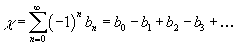
The Euler characteristic of any topological space is defined as an alternating sum of its Betti numbers.
χ = b0 - b1 + b2 - b3 +...
Here are the Euler characteristics for the manifolds listed above.
1. χ(S1) = 1 - 1 + 0 - 0 +... = 0
2. χ(T2) = 1 - 2 + 1 - 0 + 0 - ... = 0
3. χ(T3) = 1 - 3 + 3 - 1 + 0 -... = 0
4. χ(Rn) = 1 - 0 + 0 - 0 + 0 -... = 1
5. χ(CP∞) = 1 - 0 + 1 - 0 + 1 -...= ∞
In my paper "Beyond the Standard Model", I give the Betti numbers and Euler characteristic of a Calabi-Yau manifold.
If the topology is approximated by CW-complex, the above definition reduces to the alternating sum
χ = k0 - k1 + k2 - k3 +...
where k is the number of cells of dimension n in the complex.
A polytope is a type of CW-complex, where the manifold it approximates is Sn. A polyhedron is a CW-complex where k0 is the number of vertices, k1 is the number of edges, and k2 is the number of faces. The above formula then reduces to

χ = V - E + F
where V is the number of vertices, E is the number of edges, and F is the number of faces. Polyhedra are homeomorphic to a sphere, S2, which has an Euler characteristic of 2, so therefore

V - E + F = 2
which is the original Euler's formula. This famous formula was discovered by Leonard Euler (1707 - 1783), one of the greatest mathematicians. Originally from Switzerland, he went to St. Petersburg at the request of Catherine the Great, who also hosted the mathematician Dennis Diderot, and corresponded with Voltaire. Euler then went to Prussia, and served as mathematician for Frederick the Great. After he lost sight in one of his eyes, Frederick called him his "mathematical cyclops". Euler returned to St. Petersburg where he went completely blind. Incidentally, Voltaire also had an adulterous affair with Emily du Chatalet who, as one of the few female scientists before the late 19th Century, helped determine that the energy of a body is proportional to its velocity squared.
The Euler characteristic of a compact 2D manifold can be calculated from
χ = 2 - 2g - b - k
where g is the genus or number of handles, b is the number of boundaries, and k takes into account the possibility of the manifold being non-orientable. The genus g is technically defined as the number of tori in a connected sum of the surface. Similarly, k is the number of projective planes in a connective sum of the surface.
Here are some examples.
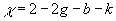
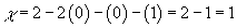
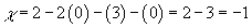
1. For sphere, S2, you have
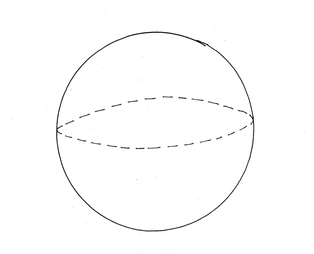
χ = 2 - 2g - b - k
χ = 2 - 2(0) - (0) - (0) = 2
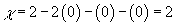
2. For a torus, T2, you have
χ = 2 - 2g - b - k
χ = 2 -2(1) - (0) - (0) = 2 - 2 = 0
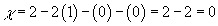
3. For a finite cylinder, S1 x I, you have
χ = 2 - 2g - b - k
χ = 2 -2(0) - (2) - (0) = 2 - 2 = 0
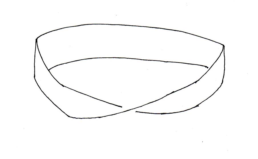
4. For a Klein bottle, KB, you have
χ = 2 - 2g - b - k
χ = 2 - 2(0) - (0) - (2) = 2 - 2 = 0
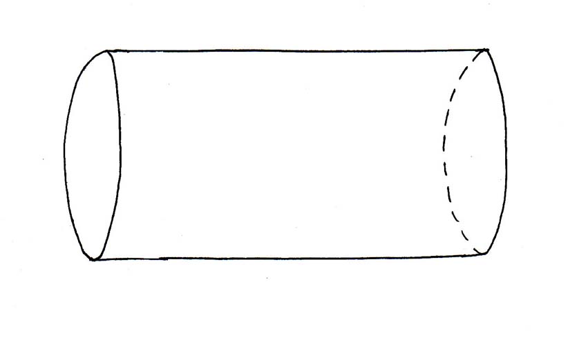
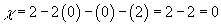
5. For a Möbius strip, MS, you have
χ = 2 - 2g - b - k
χ = 2 - 2(0) - (1) - (1) = 2 - 1 - 1 = 0
6. For a Roman surface, you have
χ = 2 - 2g - b - k
χ = 2 - 2(0) - (0) - (1) = 2 - 1 = 1
7. For a double torus, T2 # T2, you have
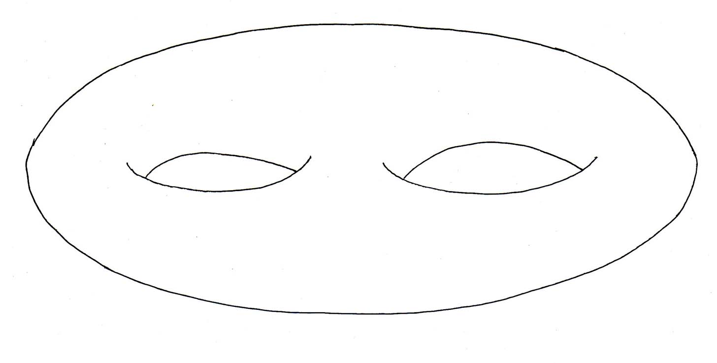
χ = 2 - 2g - b - k
χ = 2 - 2(2) - (0) - (0) = 2 - 4 = -2
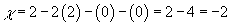
8. For a "pair of pants", you have
χ = 2 - 2g - b - k
χ = 2 - 2(0) - (3) - (0) = 2 - 3 = -1
The Euler characteristic of the disjoint union of two unconnected manifolds is simply the sum of their Euler characteristics, so the Euler characteristic of two spheres is 2 + 2 = 4.
Let's go back to this definition.
χ = b0 - b1 + b2 - b3 +...
Any contractible space Rn has trivial homology, meaning the 0th Betti number is 1, and all others 0. Therefore, its Euler characteristic is 1. This includes Rn of any dimension, as well as finite subgroups thereof, such as interval, disk, ball, etc. Any polytope of any dimension, such as any point, line segment, polygon, polyhedron, polychoron (4D polytope), etc, as well as any finite lattice thereof, such as a checkerboard, Rubik’s cube, finite honeycomb, kagome lattice, etc, will obey
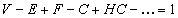
V - E + F - C + HC - ... = 1
where V is the number of vertices, E is the number of edges, F is the number of faces, C is the number of cells, HC is the number of hypercells, etc, as long as you count the interior, so a line segment would be considered to have one edge, a polygon would be considered to have one face, a polyhedron would be considered to have one cell, etc. In that case, the polytope or finite lattice would be topologically equivalent to a finite subunit of Rn, such as a disk or ball, and would therefore have an Euler characteristic of 1. If you take the absolute value of series, then it will also work for any Rn, such as a point, line, plane, 3D space, 4D space, etc, as well unbounded polytopes, such as a wall, chimney, etc.
In homology, if (dn : An → An - 1) is a chain complex such that all but a finitely many An are zero, and the others are finitely generated abelian groups, or finite dimensional vector spaces, then you can define the Euler characteristic as
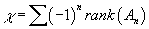
χ = [summation] (-1)n rank (An)
using the rank in the case of the abelian groups, or the Hamel dimension in the case of vector spaces. It turns out that the Euler characteristic can also be computed at the level of homology.
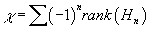
χ = [summation] (-1)n rank (Hn)
This provides two ways to compute χ for the object X which gave rise to the chain complex. Every short exact sequence
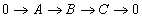
0 → A → B → C → 0
of chain complexes gives rise to a long exact sequence of homology groups

...→ Hn(A) → Hn(B) → Hn(C) → Hn – 1(A) → Hn – 1(B) → Hn – 1(C) → Hn – 2(A) → ...
All maps in this long exact sequence are induced by the maps between the chain complexes, except for the maps Hn(C) → Hn - 1 (A). These are called connecting homomorphisms and are provided by the snake lemma.
If X is a topological space, and ABC ⊂ X are such that X = int (A) ∪ int (B) and C = A ∩ B, then there is an exact sequence of homology groups

...→ Hn(C) → Hn(A) + Hn(B) → Hn(X) → Hn – 1(C) →...
where i* is induced by the inclusions i : B → X and j* by j : A → X, and ∂* is the following map. If X is in Hn(X), then it can be written as a sum of a chain in A, and one in B, x = a + b, ∂x = -∂b, since ∂x = 0. Thus, ∂a is a chain in C, and so is a class in Hn - 1(C). This is ∂*X. You can easily check by standard diagram chasing that this map is well defined on the level of homology. This sequence is called the Mayer-Vietoris sequence.
The Mayer-Vietoris sequence, named after Walter Mayer and Leopold Vietoris, is an exact sequence that you can use to compute homology groups. It's somewhat analogous to the Siefert-van Kampen theorem for homotopy groups. Homology groups can be computed directly using the tools of linear algebra in simplicial homology. However, such calculations can be very cumbersome, and it's great to have a way to compute homology groups from other ones that you already have. The Mayer-Vietoris sequence is the easiest way to do this.
For a topological space X with two subsets U and V, whose union is X, we call (X, U, V) a triad. It's sometimes possible to form triads out of non-open subsets but it doesn't always work. The Mayer-Vietoris sequence of the triad (X, U, V) is a long exact sequence which relates the singular homology groups of the space X to those of U, V, and their intersection A.

...→ Hn + 1(X) →(∂) Hn(A) →(φ) Hn(U) + Hn(V) →(ψ) Hn(X) →(∂) Hn – 1(A) → ...
where Hn(X) is the n-dimensional homology group of the space X. The maps between each homology group of the same dimension n are induced by the inclusions of A into U, and U and V into X. More precisely, the map φ into the direct sum is a product map, and the map ψ out of the direct sum is a difference. The map ∂ that lowers the dimension is a boundary map that comes from the snake lemma.
One application of the Mayer-Vietoris sequence is to prove that the n-th reduced homology group of the sphere Sk is trivial unless n = k, in which case Hk(*Sk) is isomorphic to the group of integers Z. Here you have a complete classification of homology groups for spheres, in contrast to what is known for the homotopy groups of spheres. There is a similar result for n < k, but not much is known for n > k.
The morphisms in homology are called functors. A functor is a special type of mapping between categories. A covariant functor, which is what people mean when they just say "functor", is defined as follows.
Let C and D be categories. A functor F from C to D is a mapping that
1. Associates to each object X in C an object F(x) in D.
2. Associates to each morphism f : X → Y in C, a morphism F(f) : F(X) → F(Y) in D.
such that the following two properties hold
1. F(idX) = idF(X) for every object X in C.
2. F(g o f) = F(g) o F(f) for all morphisms f : X → Y and g : Y → Z.
In other words, functors preserve identity morphisms and composition of morphisms.
So you see that a functor just says that for every object and morphism in one category, you have a corresponding object and morphism in the other category. A contravariant functor, also called a cofunctor, is the same except the corresponding morphism in the other category goes in the opposite direction, from Y to X instead of X to Y.
Let C and D be categories. A contravariant functor F from C to D is a mapping that
1. Associates to each object X in C an object F(x) in D.
2. Associates to each morphism f : X → Y in C, a morphism F(f) : F(Y) → F(X) in D.
such that the following two properties hold
1. F(idX) = idF(X) for every object X in C.
2. F(g o f) = F(g) o F(f) for all morphisms f : X → Y and g : Y → Z.
In other words, cofunctors preserve identity morphisms and composition of morphisms.
You can also define a contravariant functor as a covariant functor on a dual category Cop. Some people prefer to write all expressions covariantly, so instead of saying F : C → D is a contravariant functor, they would say F : Cop → D or F : C → Dop and call it a covariant functor.
The different types of categories that functors act on could be sets, represented by "Set", categories, represented by "Cat", groups, represented by "Grp", abelian groups, or "Ab", rings or "Rng", group homomorphisms or "Hom", topology or "Top", algebra or "Alg", etc. For instance, λCalc → Cart is a functor from a typed λ-calculus to a cartesian closed category. Top → Phas is a functor from a target space to a phase space. 2Cob → VectK is a functor from the category of 2-dimensional cobordisms to the category of vector spaces over K.
Forgetful functors are functors that go from an object with more structure to an object with less structure, so it "forgets" some structure. One example is the functor U : Grp → Set, which maps from a group to a set. In other words, it "forgets" the binary operation, leaving only the members of the group, which without a binary operation, now form a set. Another example is the functor Rng → Ab, which maps from a ring to its underlying abelian group. Going in the opposite direction from forgetful functors are free functors. The free functor Set → Grp sends every set X to the free group generated by X. Functions get mapped to group homomorphisms between free groups. The extra structure that is added during the morphism is unspecified by the original and is thus "free" to take any value.
To every pair A, B of abelian groups, you can assign the abelian group Hom(A, B) consisting of all group homomorphisms from A to B. This is a functor which is contravariant in the first, and covariant in the second, argument. It is a functor Abop x Ab → Ab where Ab denotes the category of abelian groups with group homomorphisms. If f : A1 → A2 and g : B1 → B2 are morphisms in Ab, then the group homomorphism Hom(f, g) : Hom (A2, B1) → Hom(A1, B2) is given by φ | → g o φ o f.
You can generalize this is any category C. To every pair X, Y of objects in C, you can assign the set Hom(X, Y) of morphisms from X to Y. This defines a functor to Set which is contravariant in the first argument, and covariant in the second argument. This is a functor Cop x C → Set. If f : X1 → X2 and g : Y1 → Y2 are morphisms in C, then the group homomorphism Hom(f, g) : Hom(X2, Y1) → Hom(X1, Y2) is given by φ | g o φ o f.
If X is a topological space, then the open sets in X form a partially ordered set Open(X) under inclusion. Like every partially ordered set, Open(X) forms a small category by adding a single arrow U → V if and only if U is a subset of V. Contravariant functors on Open(X) are called presheaves on X. For instance, by assigning to every open set U the associative algebra of real-valued continuous functions on U, you get a presheaf of algebras on X.
On any category C, you can define the identity functor 1C, which maps every object and morphism to itself. You can also define the constant functor, C → D which maps every object in C to a specific object X in D, and every morphism in C to the identity morphism on X. You can compose functors. If F is a functor from A to B, and G is a functor from B to C, then you can form the composite functor GF from A to C. Composition of functors is associative where defined. This shows that functors can be considered as morphisms in categories of categories.
Functors themselves can be considered as objects in a category called a functor category. Morphisms in this category are natural transformations between functors. You can then have functors acting between functor categories. The diagonal functor is defined as the functor from D to the functor category DC which sends each object in D to the constant functor at that object.
Chain complexes form a category. A morphism from the chain complex dn : An → An – 1 to the chain complex en : Bn → Bn – 1 is sequence of homomorphisms fn : An → Bn such that fn – 1 * dn = en – 1 * fn for all n. The n-th homology Hn can be viewed as a covariant functor from the chain complexes to the category of abelian groups.
If the chain complex depends on the object X is a covariant manner, meaning that any morphism X → Y induces a morphism from the chain complex of X to the chain complex of Y, then the Hn are covariant functors from the category it belongs to into the category of abelian groups.
In homology, the chain complexes depend in a covariant manner on X, and the homology groups form covariant functors. If instead, you assume that the chain complexes depend in a contravariant way on X, the homology groups form contravariant functors. The resulting subject is called cohomology. When you go from covariant functors to contravariant functors, you go from homology to cohomology. You refer to the chains as cochains, and the groups as cohomology groups. Cohomology can be viewed as a method of assigning algebraic invariants to a topological space that has a more refined structure than does homology. Cohomology arises from the algebraic dualization of the construction of homology. Homology and cohomology are duals of each other. You could also say that the cochains in cohomology should assign quantities to the chains in homology.
Homology began in the late 19th Century. They thought of a k-chain as a formal combination

[summation] aidi
where ai are integers, and di are k-dimensional simplices on X. For instance, if X is a two-torus T2, a one-dimensional cycle on T2 is intuitive in terms of a linear combination of curves drawn on T2, which closes up on itself, obeying the cycle condition, meaning having no boundary. If C and D are cycles each wrapping once around T2 the same way, you can find an oriented surface on T2 with boundary C-D. Topologists can prove that the homology classes of 1-cycles with integer coefficients form a free abelian group with two generators, one for each of the two different ways around a torus.