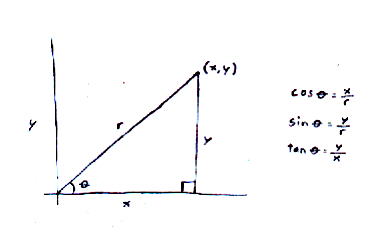
Let's review the definitions of trigonometric functions. Let's say you have a right triangle, with the small point at the origin. The angle at that point is θ, the horizontal line is x, the vertical line is y, and the diagonal line is r.
cos [theta] = x/r
sin [theta] = y/r
tan [theta] = y/x
Often it is convenient to change the axes of the coordinate system you are using. When you change the axes, the coordinates are different.
In three dimensions, the new coordinates are given by
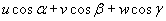
u cos [alpha] + v cos [beta] + w cos [gamma]
If you use l, m, and n to mean the cosines of the angles between the old and new axes, you have
ul + vm + wn
You can simplify it further by calling the coefficients u1, u2, and u3, and the cosines of the angles l1, l2, l3

[summation of] ui li where i = 1, 2, 3
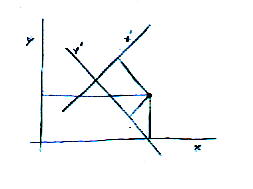
Let's say you have two sets of axes. The first is xi. The second is xj' and has the same origin as xi, just rotated.
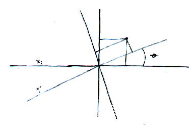
Here I've drawn it as two dimensions but let's say you have the same thing in three dimensions.
How do you change the coordinates from one system to another? Just multiply by the cosine of the angle between them.
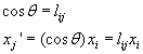
cos [theta] = lij
xj' = (cos [theta]) (xi) = lijxi
which is the same going back, so
xi = lijxj'
This formula works not just for position but for displacement, velocity and acceleration. It also works for force as long as the equations of motion are true in all reference frames. You can break this apart into each of the coordinates of the point. In three dimensions, there are three equations, each of which have the following form:
Aj' = lijAi or
Ai = lijAj'
Together, these three equations comprise the components of a vector. This is what defines a vector. The rotation and translation of axes can be drawn like this.
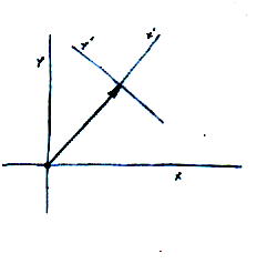
This is why a vector can also be drawn as an arrow.
This is a vector.
xj' = lij xi
xi = lij xj'
These are the components of a vector.
Aj' = lij Ai
Ai = lij Aj'
Let's say you were to have two of each of the variables.
Aj' Bl' = lijlkl Ai Bk
AiBk = lijlkl Aj' Bl'
These are the individual components, and if you combine them you have this.
kjl' = lijlkl kik
kik = lijlkl kjl'
This is called a second order tensor. You cannot draw it geometrically like you can a vector but you can deal with it algebraically as easily as a vector. A scalar is a zero order tensor. A vector is a first order tensor. This is a second order tensor, which is also called a dyad. In physics, you frequently use second order tensors. Rarely, you use third and fourth order tensors. You almost never use higher orders, although mathematically you could have any order by just having higher multiples of the number of variables.
If you look at the tensor kik, you see there are two subscripts, each of which could have values 1, 2, or 3. Therefore, there are 32 = 3 x 3 = 9 combinations. For this reason, the tensor can be written as a matrix.
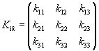
            k11  k12  k13
K =         k21  k22  k23
            k31  k32  k33
Even though it's a 3 x 3 matrix, it's a second order tensor, since k has two subscripts.This is a common notation for tensors. The components k11, k22, and k33 are called the diagonal. Often you have zeroes off the diagonal. The sum of the components of the diagonal is called the trace or spur.
(K + L)ik = Kik + Lik which is a tensor
Kjl' = likljl Kik

likljl = [delta]ik which is the same for any rotation
δik is an isotropic tensor which means it is unaltered by rotation. There are no isotropic tensors of the first order. The only isotropic second order tensors are multiples of δik. The only isotropic third order tensors are multiples of εikm. There are three independent ones of the fourth order which are

[delta]ik[delta]mp
[delta]im[delta]kp + [delta]ip[delta]km
[delta]im[delta]kp - [delta]ip[delta]km
It's possible to multiply a tensor by a vector, and then write it in dyadic notation.
A.K = AiKik or K.A = KikAk
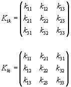
If you have a tensor Kik and you exchange rows and columns, you get another tensor Kki.
If Kik = Kki, the tensor is symmetrical. If Kik = - Kki, the tensor is antisymmetrical. If Kik is a tensor, two others are Kik + Kki and Kik - Kki. The first of these is unaltered if i and k are exchanged and is a symmetrical tensor. The second has all the components reversed, and is an antisymmetrical tensor. Any tensor Kik can be written as the sum of a symmetrical and antisymmetrical tensor.
Kik = 1/2(Kik + Kki) + 1/2(Kik - Kki)
The diagonal components of an antisymmetrical tensor Kik must vanish, and since for the others Kik = -Kki, only three independant quantities are needed to specify an antisymmetric tensor, which then takes the form
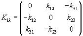
              0        K12    -K31
Kik =        -K12      0       K23
              K31     -K23     0
If Kik = -Kki, then K11 = - K11, K22 = - K22, and K33 = - K33, which is only true if K11 = K22 = K33 = 0.You now have three values, K12, K23, and K31. However, the vector Ki, where i has a value for each of the three axes, x, y, and z, also has three values. Therefore these three values can be used to define a vector. Therefore, an antisymmetrical tensor can be written as a vector.
δik is the Kronecker delta, and in Euclidean space, is equal to the metric tensor. εikm is the permutation tensor.
Sometimes vectors can be most simply written in tensor notation. For instance, the dot product between two vectors can be simply written as

u . v = ui vi
where repeated indices are summed so that
ui vi = u1 v1 + u2 v2 + . . . um vm
The cross product of two vectors can be written as

u x v = [epsilon]ikm uj vk
A vector is usually portrayed as a 1 x n matrix. If it's portrayed as a m x 1 matrix, it's called a column vector. A two-component complex column vector is called a spinor. It's actually much more complicated than that, but this is sufficient for our present purposes. Here's a typical spinor describing a fermion of arbitrary helicity.

In cosmology, the structure of spacetime is described by a metric. The simplest is flat spacetime which is described by the Minkowski metric, which is as follows.
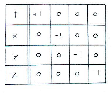
Minkowski metric, guv
t -  +1  0  0  0

x-    0 -1  0  0

y-    0   0 -1 0

z-    0   0  0 -1
This is a second order tensor where the upper left hand value is +1, the other values in the diagonal are -1, and you have zeroes off the diagonal. The Minkowski metric is represented by guv or guv = Diag[+1, -1, -1, -1]
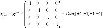
Notice that the time coordinate is +1, and the three spatial coordinates are -1. Some people use an opposite sign convention with the time coordinate -1, and the space coordinates +1. When a tensor used in physics has the form of the first coordinate being the time coordinate, and the remaining three being spatial coordinates, with zeroes off the diagonal, it's called a 4-vector. Technically, it's a second order tensor but you could pretend it's a vector with four components, t, x, y, and z. A 4-vector has the following general form.
Au = (at, ax, ay, az) = (a0, a1, a2, a3) = (a0, a)
Since the three spatial components are often exactly the same, they are often represented by a single boldface variable a1, a2, a3 = a. It's also sometimes represented by a variable with an arrow over it.

If you multiply a 4-vector times the Minkowski metric guv, this has the effect of putting a minus sign on the space part. The result is called a 4-covector, and you switch from superscripts to subscripts.
guvAu = Au = (at, -ax, -ay, -az) = (a0, -a1, -a2, -a3) = (a0, -a)
In flat space, the Minkowski metric guv is the same as the metric tensor, which is actually a function that computes the distance between two points in general space. It's derived from a generalization of the Pythagorean theorem. In curved space, meaning in the presence of a gravitational field, the metric tensor has to be a coordinate dependent field transforming in the right way to keep the proper time invariant.
In Newtonian mechanics, you can change from one inertial frame to another by translations and rotations. This is only within the three spatial coordinates since time is not included. In special relativity, you can change from one inertial frame to another within not just space but spacetime, so all four coordinates are included. You have the translations. You also have a group of transformations called Lorentz transformations, which include rotations and boosts, which are changing from a motionless inertial frame to one moving at a constant velocity. The translations and Lorentz transforms together form the Poincare transforms. If something is unchanged under Lorentz transforms, it's Lorentz invariant. If it's unchanged under Poincare transforms, it's Poincare invariant.
4-vectors are Poincare invariant. That means they are valid in all inertial frames regardless of coordinate system. The components might change from one reference frame to another but the 4-vector is not changed. It's valid for all inertial observers. Luv is the Lorentz transform. It is a transformation tensor that gives relations between different inertial reference frames.
A'u = Luv Av
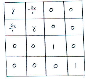
Lorentz transform, Luv
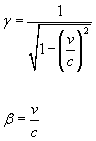
[gamma]      -[gamma]v/c        0            0

[gamma]v/c    [gamma]           0            0

0               0               1            0

0               0               0            1
where γ is the Lorentz factor, γ = 1/[squareroot of (1 - (v/c)2)] Also β = v/c
From this, you get the relation between a given quantity at rest, and then its measured relativistic value.

length L = L0/[gamma]

time t = [gamma]t0
volume V = V0/[gamma]
temperature T = T0/[gamma]
heat Q = Q0/[gamma]
entropy density S = [gamma]S0
Some quantities are unchanged, such as pressure and entropy.
Usually 4-vectors contain only real components. However, it is possible for them to contain imaginary components. An example is the polarization 4-vector.
i = [squareroot of -1] All complex numbers have the form a + bi. For non-imaginary real numbers, b = 0. For imaginary numbers, b is not 0. For pure imaginary numbers a = 0. If you have a number a + bi, the complex conjugate of the number is a - bi. Here is the general form of a 4-vector.
A = (a0, a)
If you take into account imaginary numbers, it becomes
A = (a0r + ia0i, ar + iai)
We use the subscripts r and i to keep track which are real versus imaginary. The complex conjugate of the 4-vector A is as follows.
A = (a0r - ia0i, ar - iai)
The 4-vector is frequently used in physics. Here is list of some 4-vectors. [h bar] = h/2π where h is Planck's constant. h = 6.626 x 10⁻³⁴ Js. 1 joule = 1 kgm2/s2. c is the speed of light, which is the velocity of a massless particle from the reference frame of a particle with mass. c = 2.99792458 x 10⁸ m/s. m0 is the rest mass of a particle, and q0 is the charge of a particle. I give the 4-vector, how it's defined, and then its units. These are all Lorentz vectors.
4-vector - definition A = (a0, a) - (SI units)
4-position - R = (ct, r) - (m)
4-velocity - U = γ(c, u) - (m/s)
4-acceleration - A = γ(dγ/dt c, dγ/dt u + γa) - (m/s2)
4-momentum - P = (E/c, p) = γm0(c, u) = m0U - (kgm/s)
4-force - F = γ(dE/cdt, f) - (kgm/s2)
4-displacement - dR = (cdt, dr) - (m)
4-wave vector - K = (w/c, k) = (w/c, wvphasen) = 1/[h bar] (E/c, p) - (rad/m)
4-current density - J = (cp, j) = p0γ(c, u) = p0U - (C/m2s)
4-number flux - N = γn0(c, u) = n0U - (m/s)
4-polarization - E = (e0, e) - (none since it contains imaginary components)
4-gradient - d = d/dxu = (d/cdt, [nabla]) - (1/m)
4-vector potentialEM - AEM = (VEM/c, aEM) - (kgm/Cs)
4-momentumEM - PEM = (E/c + qVEM, p + qaEM) - (kgm/s, including EM potentials)
4-gradientEM - D = (d/dct + iq/[h bar](VEMc), -[nabla] + iq/[h bar]aEM) - (1/m, including EM potentials)
If you multiply the 4-gradient by itself you get
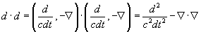
dd = (d/cdt, [nabla]).(d/cdt, [nabla]) = (d2/c2dt2)-[nabla].[nabla]
This is known as the D'Alambertian operator. It is usually symbolized by a square. It was invented by D'Alambert. Who invented the Fourier series? This might sound like a self-evident question but remember that Monroe was not responsible for the Monroe Doctrine. D'Alambert did work on the vibrating string, and in the process of that he and Euler came up with the Fourier series in 1747. D. Bernoulli got the solution as a sine series in 1753, and what we call the Fourier sine theorem followed from that. Fourier tried to prove it in his work on heat conduction titled, "Analytical Theory of Heat" published in 1822, but the attempt at a proof was inaccurate and almost incoherent. It was actually proven by Dirichlet in 1829.
You use tensors to provide generally valid relations between 4-vectors. Since the components of 4-vectors are altered by change of axes, the components of tensors have to be able to change also, so they can still provide relations between the same 4-vectors. Here is the tensor transformation law.
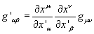
g'[alpha][beta] = [partial derivative of xu with respect to x'[alpha]] [partial derivative of xv with respect to x'[beta]]guv
For Cartesian coordinates, it would make no difference if we turn the fractions upside-down.
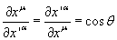
[partial derivative of xu with respect to x'[alpha]] = [partial derivative of x'[alpha] with respect to xu] = cos [theta]
where θ is the angle of rotation between the two axes. However, this is not in general true.
If you have the 4-vector Au, the components are xu = (ct, -x, -y, -z). These are the covariant components of Au. They transform the same way as a vector. If you multiply by the metric tensor, you get xu = (ct, x, y, z) which are the contravariant components of the 4-vector Au. They transform oppositely of a vector.
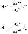
A'u = [partial derivative of x'u with respect to xv]Av
A'u = [partial derivative of xv with respect to x'u]Av
It is also possible to contract tensors. If you multiply Au by Au, you get a scalar. The process is called contracting, and the result is called the size or norm of the tensor Au. Au Au is invariant. Au Au would not be a constant. The effects of arbitrary coordinate changes do not cancel unless you have upstairs and downstairs indices.
Let's say you have Au Bu = 1, and Au is a 4-vector. Therefore, Bu must also be a 4-vector in order for the right hand side to be a scalar. This method of deducing the nature of the quantities in an equation is called manifest covariance.
A coordinate derivative is when a derivative acts on a single coordinate.

The index must be downstairs since the derivative acts on only one coordinate.
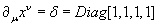
[coordinate derivative of u on xv] = [delta] = Diag[1, 1, 1, 1]
Notice we once again see δ, which is an isotropic tensor, meaning that components are the same in all frames. It must exist in order to define the inverse matrix of a tensor. If you have both a partial derivative with upstairs indices and a partial derivative with downstairs indices, you have the D'Alambertian operator.

The scalar product of two 4-vectors is
au bu = a0 b0 - a1 b1 - a2 b2 - a3 b3
The metric tensor is a tool used to raise and lower indices.
Au = guv Av
For example, in special relativity, the 4-derivatives are
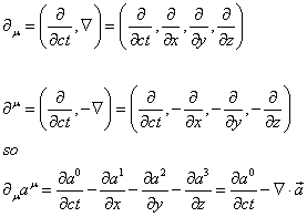
[partial derivativeu] = ([partial derivative with respect to ct], [nabla]) = ([partial derivative with respect to ct], [partial derivative with respect to x], [partial derivative with respect to y], [partial derivative with respect to z])
[partial derivativeu] = ([partial derivative with respect to ct], -[nabla]) = ([partial derivative with respect to ct], -[partial derivative with respect to x], -[partial derivative with respect to y], -[partial derivative with respect to z])
so therefore [partial derivativeu]au = [partial derivative of a0 with respect to ct] - = [partial derivative of a1 with respect to x] - = [partial derivative of a2 with respect to y] - = [partial derivative of a3 with respect to z] = [partial derivative of a0 with respect to ct] + [nabla]a
Therefore conservation laws, such as for the 4-current, can be written as ∂uJu = 0.

Tensor equations with indices in the same relative positions on either side must be generally valid. The equation is called generally covariant. This has nothing to do with the word "covariant" in "covariant components".
The determinant of a tensor is defined as follows.
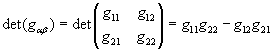
det(g[alpha][beta]) =
|g11 g12| | | = |g21 g22|g11 g22 - g12 g21
since in matrices
|a           b|
|             | =  ad-bc
|c           d|
g = -detguv
Then you have
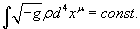
[integral of] [squareroot of -g]pd4xu = constant
[squareroot of -g]is called the Jacobian. For Minkowski spacetime, g is -1, so the Jacobian is +1 or -1. [squareroot of -g]p is the scalar density. An object formed from a tensor and n powers of the squareroot of -g is called the tensor density of weight n.
If the Jacobian is positive, that is called a proper transformation. If the Jacobian is negative, that is called an improper transformation. In special relativity, a tensor density will transform like a tensor if you restrict yourself to proper transformations. However, with improper transformations, or spatial inversion, tensor densities of odd weights will change sign. These quantities are called pseudotensors. Pseudotensors include pseudovectors and pseudoscalars. The most famous example is the antisymmetric Levi-Civita tensor, εαβγδ.

[epsilon][alpha][beta][gamma][delta] = g[epsilon][alpha][beta][gamma][delta]
It is equal to +1 if the indices are an even permutation of 0123, and -1 if they are an odd permutation. It's 0 for any other value of indices. Here, a "permutation of 0123" is an ordering of the numbers 0, 1, 2, 3 which can be obtained by starting with 0123 and exchanging two of the digits. An even permutation is obtained by an even number of such exchanges, and an odd permutation is obtained by an odd number.
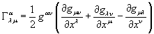
The Christoffel symbol of the first kind is represented in various ways including
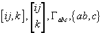
These are called components of the affine connection. They are defined by
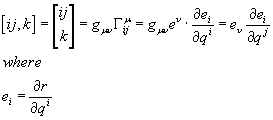
[ij, k] =
| ij| = | k|guv[Christoffel symbol, capital gamma]uij = guveu [partial derivative of ei with respect to qi] = ev [partial derivative of ei with respect to qi]
where guv is the metric tensor and ei = [partial derivative of r with respect to qi]
Here is the Christoffel symbol expressed in terms of the metric tensor.
The following define the covariant derivative.
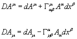
DAu = dAu + [Christoffel symbol]u[alpha][beta]A[alpha]dx[beta]
DAu = dAu - [Christoffel symbol][alpha]u[beta]A[alpha]dx[beta]
You can generalize equations by replacing ordinary derivatives by covariant derivatives. The equation of motion for a particle would become

Fu = m(DUu/d[tau])
In order to simplify the notation, partial derivatives are often represented by a comma. Covariant derivatives are often represented by a semicolon.
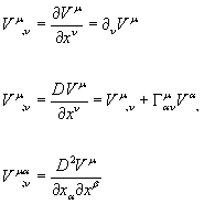
Vu,v = [partial derivative of Vu with respect to xv] = [partial derivativev Vu]
Vu;v = DVu/[partial derivative]xv = Vu,v + [Christoffel symbol]u[alpha]vV[alpha],
For instance, for Maxwell's equations, you have Fuv;v = -u0Ju
In physics, you frequently use the energy-momentum tensor Tuv. Its value depends on the system. For instance, for a cold fluid with density p0 in its rest frame, the only non-zero component is the upper left T00 = c2p0 In a general frame, you have
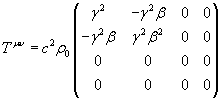
TUV = c2p0
[gamma]^2               -[gamma]^2[beta]           0            0

-[gamma]^2[beta]        -[gamma]^2[beta]^2         0            0

  0                       0                        0            0

  0                       0                        0            0
where β = v/c and γ = 1/[squareroot of 1 - (v/c)2]. This is similar to the Lorentz transform. You have two powers of γ, one for the change in number density, and one for the relativistic mass increase. For a perfect fluid, the rest-frame Tuv is
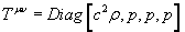
Tuv = Diag[c2[rho], p, p, p]
In a general frame, the energy momentum tensor of a perfect fluid is
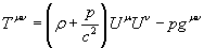
Tuv = ([rho] + p/c2)UuUv - pguv
In order to explain the fact the Universe is homogeneous and isotropic, we invented inflation which predicted that the universe is flat. Fortunately for us, we observed that the universe is flat since the cosmic microwave background is isotropic. However, then we determined that the amount of matter in the Universe was insufficient to cause the Universe to be flat. We then had to invent some sort of dark energy to flatten the universe. However, this dark energy would also predict that the universe is accelerating. Then Hubble measured the redshift of distant supernovae and determined that the expansion of the Universe really is accelerating, so it's consistent. Primary candidates for the dark energy are the cosmological constant, a rolling scalar field called quintessence, or topological defects.
In 1998, a balloon called Boomerang floated around Antarctica for ten days, and measured the anisotropy of the cosmic microwave background to high precision. The conclusion is that the Universe is very close to flat.
However, on small scales, the Universe is curved. General relativity uses this curvature to explain gravitational effects. The Minkowski metric describes flat spacetime. How do you describe curved spacetime?
In 1884, Erwin A. Abbott wrote a book titled "Flatland" about two dimensional creatures. If a group of such creatures were living on the surface of a large sphere, how would they know it wasn't a plane? Gauss was the first to recognize that you could do this by measuring the angles of a triangle. The angles of a triangle on a plane, or in Euclidean space, always add up to 180o or π radians. The angles of a triangle on a positively curved surface, such as a sphere, add up to more than that. The angles of a triangle on a negatively curved surface, such as a saddle surface, add up to less than that.
This is actually a specific example of a more general case called parallel transport. Imagine that you have a square on a plane. If you move a vector around this square, it's always either parallel or perpendicular to the line it's on. The vector is always facing in the same direction. Let's say you do the same thing with a triangle on a sphere where each of its angles are 90o. You can get the vector pointing in different directions depending on which direction it takes around the triangle.
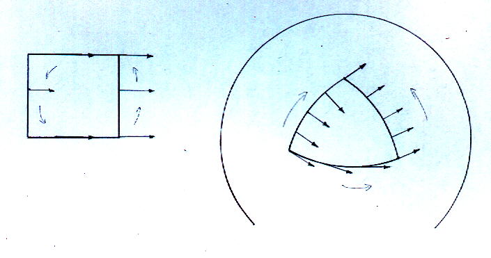
Take the path integral around the loop. The extent of curvature is the change in the vector which is proportional to both the vector itself, due to rotation, and the distance along the loop, to first order, so that the total change in going around a small loop is given by

[delta]Vu = '[Ru[alpha][gamma][beta] [path integral ([capital delta]x[beta]dx[alpha] - [capital delta]x[alpha]dx[beta])]]
Since Γ is a function of position in the loop, it can't be taken out of the loop. Make first order expansions of Vu and Γ as functions of the total displacement from the starting point Δxu. For Γ, the expansion is a first-order Taylor expansion. For Vu, what matters is the first order change in Vu due to parallel transport.
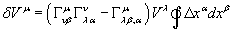
There's no first order term because

around the loop. Writing this twice and permutating α and β gives you
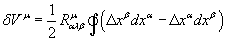
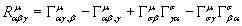
where Ruαγβ is the Riemann tensor. The Riemann tensor Ruαγβ is defined as
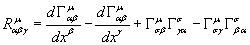
which can be written as
The Riemann tensor is a fourth order tensor. However, if you multiply Au by Au, you get a scalar. Au = guvAu. In this way, you can reduce a fourth order tensor to a second order tensor.
Ruv = R[gamma]u Ru[alpha][gamma][beta]
Ruv is the Ricci tensor. You can do the same thing again and contract it to the curvature scalar R.
R = RuvRuv
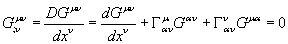
The following is the Einstein tensor Guv.
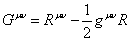
Guv = Ruv - (1/2)guvR
Notice that the Einstein tensor has zero covariant divergence.