
An integral of a function is the area under a curve described by that function. Let's say you have the following integral.
S = [integral] f(dx/dt, x, t)dt
where f is a function, and x is a function of t
What function does x have to be so that S will remain stationary for small changes in x? This type of problem is called the calculus of variations. The simplest example is what is the shortest path between two points. We know the answer is a straight line. Let's say you define a function x'(t) that is slightly different then x(t)
x’(t) = x(t) + [delta]x(t)
where [delta]x(t) = [alpha]g(t)
x(t) makes the integral stationary if
[partial derivative with respect to alpha][integral]f(dx'/dt, x', t)dt = 0 when [alpha] = 0
You have
[partial derivative with respect to alpha][integral]f(p + [alpha]dg/dt, x + [alpha]g(t), t)dt
= [integral] [partial derivative with respect to alpha]f(p + [alpha]dg/dt, x + [alpha]g, t)dt
= [integral](dg/dt, [partial derivative of f with respect to p] + g[partial derivative of f with respect to x])dt
You would solve this integral by integrating by parts. Let me explain what that is.
Let's say you want to integrate the following integral.

[integral]udv
Notice the following.
d(uv) = udv + vdu
[integral]d(uv) = uv = [integral]udv + [integral]vdu
Get ∫udv on one side
[integral]udv = uv - [integral]vdu
Incidentally, the minus sign we created is why you have the minus sign in the Hamiltonian and Lagrangian.
[integral]udv = [uv] - [integral] vdu where [f] = f(b) - f(a)
So now instead of having to solve for ∫udv, you have to solve ∫vdu which might be an easier integral to solve. If not, you shouldn't use parts. You might use various substitutions and parts several times in one problem. Now, let's go back and use parts on the problem we were working on.
[integral] (dg/dt [partial derivative of f with respect to p] + g[partial derivative of f with respect to x])dt
[g[partial derivative of f with respect to p] + [integral]g([partial derivative of f with respect to x] - d/dt[partial derivative of f with respect to p])dt
Lets say you have 3n functions q of the coordinates. You can write
xri = xri(q1, q2,.... q3n)
q is called generalized coordinates. A dot over a variable denotes differentiations with respect to time.
[delta]xri = [partial derivative of xri with respect to q][delta]q
[x dot]ri = [partial derivative of xri with respect to q][q dot]
[partial derivative of [x dot]ri] = [partial derivative of xri with respect to q]
2T = [summation]mr ([partial derivative of xri with respect to q][q dot])2
[summation]Xridxri = [summation]Xri[partial derivative of xri with respect to q]([delta]q) = Q[delta]q
You can then write δS as
[delta]S = [integral]([delta]T + Q[delta]q)dt
where T and Q are functions of q and [q dot]. Then you have
[integral][delta]Tdt = [[partial derivative of T with respect to [q dot]] + [[partial derivative of T with respect to q] - d/dt[partial derivative of T with respect to [q dot]][delta]qdot
The condition δS = 0 gives
d/dt [partial T with respect to [q dot]] - [partial derivative of T with respect to q] = Q
This is called Lagrange's equation. It was named after Joseph Louis Lagrange (1736 - 1813). He was a brilliant Italian mathematician who spent most of his career in Paris. He fled France during the French Revolution but returned under Napoleon. He was one of the primary architects of the calculus of variations.
This is Hamilton's principle. It was named after William Rowan Hamilton (1805 - 1865) who also invented the quaternions.
[delta]S = [delta][integral](T + W)dt = 0
where T is the kinetic energy and W is the work. The Lagrangian L can be defined as L = T + W.
[delta][integral]Ldt = [[partial derivative of L with respect to [q dot]][[delta]q] + [integral]([partial derivative of L with q] - d/dt[partial derivative of L with respect to [q dot]][delta]qdt
If t0, t1, q are varied by Δt0, Δt1, Δq, the integrated part is
[[L - q[partial derivative of L with respect to [q dot]][delta]t + [partial derivative of L with respect to [q dot]][delta]q]
since [delta]q = q + [q dot][delta]t
We define the Hamiltonian H by

H = [q dot][partial derivative of L with respect [q dot]] - L
and the canonical momentum by

p[alpha] = [partial derivative of L with respect to [q dot]]
This is Hamilton's principle function.
[delta]S = [delta][integral]Ldt = [-H[delta]t + p[alpha] [alpha]q] + [integral]([partial derivative of L with respect to [q dot]] - d/dt[partial derivative of L with respect to [q dot])[delta]qdt
You replace t1 by t, and the last integral is zero so
[partial derivative of S with respect to t) = -H
[partial derivative of S with respect to q] = p[alpha]
You can use p[alpha] = [partial derivative of L with respect to [q dot]]
to get rid of [q dot] in the Hamiltonian so
[partial derivative of S with respect to t] = -H(q, p[alpha], t)
This is called the Hamilton-Jacobi equation, first written in 1836.
L is a function of q, [q dot], and possibly t. H is a function of q, p, and possibly t. Then for variations of q and [q dot], without varying t
[delta]H = [delta]([q dot], p - L) = [q dot][delta]p[alpha] + p[alpha][delta][q dot] - [partial derivative of L with respect to q][delta]q - [partial derivative of L with respect to q dot][delta][q dot]
since
p[alpha] = [partial derivative of L with respect to q dot]
therefore
[delta]H = [q dot][delta]p[alpha] - [partial derivative of L with respect to q]q
[q dot] = [partial derivative of H with respect to p[alpha]]
[partial derivative of H with respect to q] = -[partial derivative of L with respect to q]
by Lagrange's equation
[p[alpha] dot] = d/dt[partial derivative of L with respect to q dot] = [partial derivative of L with respect to q] = -[partial derivative of H with respect to q]
therefore
[p[alpha] dot] = -[partial derivative of H with respect to q]
[q dot] = [partial derivative of H with respect to p[alpha]]
These are called Hamilton's equations.
L = T + W
Work is minus potential energy.
W = -V
therefore
L = T - V
The Lagrangian is usually described as kinetic minus potential energy.
Let's look at a simple system. One of the simplest where there is any movement at all is a harmonic oscillator. You could choose any example but let's say you have a simple pendulum that swings back and forth. What do you need to specify the state of the particle, which in this case is the bob of the pendulum? Position alone doesn't define it completely because it won't tell you whether it’s traveling to the right or left. Therefore you need the position and momentum. The momentum is defined as

p = mv = m (dx/dt)
So you need x, and the first derivative of x. The force is determined by Newton's Second Law.
F = ma = m (dx2/dt2)
In a one-dimensional simple harmonic oscillator
F = -kx, so
-kx = m (d2x/dt2)
also k/m = w2 so
-w2x = (d2x/dt2)
(d2x/dt2) + w2x = 0
The solution for position is
x(t) = A cos (wt + [theta])
The solution for momentum is
p = -mAw sin (wt + [theta])
Newton's Second Law can be written as either one second order equation or two coupled first order equations
F = dp/dt
p/m = dx/dt
For one-dimensional motion, x(t) and p(t) determine the evolution of the particle's trajectory. If you eliminate t between them, you can write p as a function of x, and derive the mechanical energy E.
p2/2m + U(x) = E
where U(x) is the potential energy. You can rewrite it as
p = ± [squareroot of] 2m(E - U(x))
If I choose any value of x, you can tell me the value of p at that position. Imagine a graph with x on the horizontal axis, and p on the vertical axis. At each instant t, the value of x corresponds to a value of p. Plot the ordered pair (x, p) on a graph. You get an ellipse.
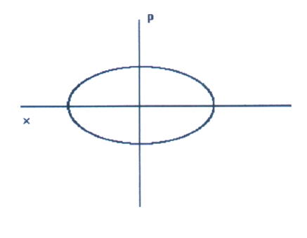
This is called phase space. As time marches on, the state point sweeps out a trajectory in phase space. The phase space trajectory of a simple harmonic oscillator forms an ellipse. The size of the ellipse is determined by the particle's energy E.
The two first order equations F = dp/dt and p/m = dx/dt describe the evolution of the phase space coordinates (x, p). These equations can be written in terms of energy instead of force. E, which appears on the right hand side of the equation, denotes the numerical value of the energy. The left hand side of the equation
p2/2m + U(x) = E
is a function of the phase space coordinates (x, p). The left hand side is the Hamiltonian of the system. If the potential energy includes an explicitly time-dependent factor, such as a spring constant that weakens with time, then the Hamiltonian H is explicitly a function of this time.
H(x, p, t) = p2/2m + U(x, t)
The equation p2/2m + U(x) = E says that the energy, a number, and the Hamiltonian, a function, have the same value. H(x, p, t) = E. For conservative systems, the force F is given as the minus partial derivative of H with respect to x.
F = dp/dt
F = -[partial derivative of H with respect to x] so
dp/dt = -[partial derivative of H with respect to x]
You can also write p/m = dx/dt in terms of H. p2/2m is the kinetic energy. Notice that
p/m = [partial derivative of H with respect to p]
p/m = dx/dt so
dx/dt = [partial derivative of H with respect to p]
Therefore you have the following two first order differential equations.
dp/dt = -[partial derivative of H with respect to x]
dx/dt = [partial derivative of H with respect to p]
These are Hamilton's equations, named after William Rowan Hamilton. They describe how the particle’s phase space point (x, p) moves with respect to time. x and p are canonically conjugate. Every position coordinate x has a specific momentum. For a particle moving in N spatial dimensions, there are 2N canonically conjugate phase space coordinates.
You can also describe the evolution of H itself. Since H = H(x, p, t), the chain rule gives
dH/dt = [partial derivative of H with respect to x](dx/dt) + [partial derivative of H with respect to p](dp/dt) + [partial derivative of H with respect to t]
When we use Hamilton's equations to write dx/dt and dp/dt in terms of derivatives of H, two terms cancel, leaving

dH/dt = [partial derivative of H with respect to t]
If you take the derivative of something with respect to something it doesn't contain, the result is zero. If H does not depend on a given variable, the partial derivative of H with respect to that variable is zero. If dH/dt = ∂H/∂t, that means H depends only on t. ∂H/∂t = 0 if and only if H contains no explicit time dependence. In other words, only when the system is invariant under time translation Δt. The momentum p is constant if and only if H does not explicitly contain its conjugate coordinate x when the system is invariant under a displacement Δx.
The Hamiltonian is rigorously approached through the Lagrangian. Newton's Second Law in generalized coordinates q, assumes the following form of the Euler-Lagrange Equation

[partial derivative of L with respect to q] = d/dt[partial derivative of L with respect to [q dot]]
where the overdot represents the time derivative. The Lagrangian L is the difference between the kinetic and potential energies, written as a function of position coordinates, velocities, and possibly the time. The Euler-Lagrange Equation can be written as
[partial derivative of L with respect to t] = -d/dt([q dot][partial derivative of L with respect to [q dot]] - L)
The last two equations follow from Hamilton's principle.

[delta][integral from a to b] Ldt = 0
Some combinations of variables occur frequently in this subject. This is the canonical momentum. It is the conjugate of the coordinate q.

p = [partial derivative of L with respect to [q dot]]
This is the Hamiltonian.

H = [q dot][partial derivative of L with respect to [q dot]] - L
The Lagrangian is a function of position and velocity. The Hamiltonian is a function of position and canonical momentum. Which you want to use depends on whether you want to use velocity or canonical momentum. H typically works out to be kinetic energy plus potential energy but it is not always the same as the energy.
Similarly, the canonical momentum is often, but not always, the mv momentum. For example, if q happens to be the polar angle θ, its conjugate momentum is the component of angular momentum about the axis of θ rotation. If a charged particle moves through an electromagnetic field, then the canonical momentum and the mv momentum differ by a vector potential term.
Hamilton's principle can be stated in terms of the Hamiltonian rather than the Lagrangian. By using the Hamiltonian
H = [q dot][partial derivative of L with respect to q dot] - L
we can rewrite Hamilton's principle
[delta][integral from a to b]Ldt = 0
as
[delta][integral from a to b][x dot]p - Hdt = 0
which gives Hamilton's equations.
Let's say you have to find the equations of motion x(t) and p(t) in a particularly difficult problem. One strategy for solving any problem is to transform it into a problem you already know how to solve. This is why you change variables. Therefore, you could try a change of phase space variables x → x', p → p', which produces a change in the Hamiltonian H → H'. Hamilton's equations hold in the new phase space as well as the old.
dx'/dt = [partial derivative of H’ with respect to p’]
dp'/dt = -[partial derivative of H’ with respect to t’]
The new Hamilton's equations are derived from minimizing the integral
[delta][integral from a to b][partial derivative of x with respect to t]’p’ - H’dt = 0
This integral must also hold.
[delta][integral from a to b][x dot]p - Hdt = 0
For the two integrals to hold simultaneously, the integrands can differ at most by a total derivative.
([partial derivative of x with respect to t]p - Hdt) - ([partial derivative of x with respect to t]’p’ - H’dt) = dS/dt
where S must include both old and new phase coordinates. It may also depend on time. Let's consider the case where S depends on the old x and new p’.
S = S(x, p', t)
From the chain rule, the above equation defining dS/dt says
0 = [ x dot]((partial derivative of S with respect to x) - p) + (H - H' + [partial derivative of S with respect to t]) + [p dot]{partial derivative of S with respect to p'] + p’([x dot]')
This equation must be true for all times and all phase space coordinates. That will happen if the grouped terms vanish separately.
p = [partial derivative of S with respect to x]
H + [partial derivative of S with respect to t] = H’
p'([x dot])’ = -([p dot])[partial derivative of S with respect to p']
We are trying to transform the problem into phase space where it becomes a problem we know how to solve. The easiest problem we know how to solve is H’ = 0. Then from Hamilton's equations, it follows that x' = constant, and p' = constant = p0.

H + [partial derivative of S with respect to t] = H’
then becomes

H + [partial derivative of S with respect to t] = 0
This is the Hamilton-Jacobi Equation (HJE). If you plug in the following definitions
H(x, p, t) = p2/2m + U(x, t)
p = [partial derivative of S with respect to x]
it becomes
p2/2m + U + [partial derivative of S with respect to t] = 0
(1/2m)[partial derivative of S with respect to x]2 + U + [partial derivative of S with respect to t] = 0
(1/2m)[partial derivative of S with respect to x]2 + U = -[partial derivative of S with respect to t]
Notice that in this form, it resembles the time-dependent Schrodinger equation.
We still haven’t actually found x(t) and p(t) so let’s do that now. We already have p from

p = [partial derivative of S with respect to x]
How do you find x? Here you have the following equation.
p'([x dot])' = -([p dot])[partial derivative of S with respect to p’]
If you impose

x’ = [partial derivative of S with respect to p’]
it requires p'x' to be constant. Therefore, to find x, you evaluate this derivative, and then set x' and p' to be constants. That will turn x' = ∂S/∂p’ into an algebraic equation to solve for x.
First you have to find S. In a typical case where H = E, the HJE
(1/2m)[partial derivative of S with respect to x]2 + U = -[partial derivative of S with respect to t]
says that S(t) ~ -Et for its time dependent part. This suggests an additive separation of variables for S
S(t, x, p0) = W(x, p0) - Et
which combined with the above equation, gives the time independent HJE
(1/2m)[partial derivative of W with respect to x]2 + U = E
that you have to solve for W.
Let’s say you have a free particle moving to the right with energy E and momentum p0 = [squareroot of 2mE]. The time independent HJE gives
[partial derivative of W with respect to x]2 = 2mE
so that W = p0x + Δ, with Δ being an arbitrary integration constant.
S(t, x, p0) = W(x, p0) - Et
We now have S.
S(t, x, p0) = p0x - ET - [delta]
S(t, x, p0) = p02/2m + [delta]
The particle’s momentum follows from p = ∂S/∂x. To obtain x(t), you use x’ = ∂S/∂p’
x' = [partial derivative of S with respect to p’] = x - (p0/m)t
set x' to a constant
x0 = x - (p0/m)t
Since there are much easier ways of doing this and other problems, the HJE is rarely used for grinding out answers to practical problems. Rather, it suggests new ways of thinking about mechanics. For instance, the HJE foreshadowed particle-wave duality.
So these are Hamilton’s equations. They are frequently used in celestial mechanics.
[q dot] = [partial derivative of H with respect to p]
[p dot] = -[partial derivative of H with respect to q]
You also have this which is related to Hamilton’s equations.

p = [partial derivative of L with respect to q dot]
H is the Hamiltonian and L is the Lagrangian.
H(q, [q dot], t) = [q dot]p - L(q, [q dot], t)
If the equations defining the generalized coordinates are not functions of time,
H = T + V = E
L = T - V
Let’s define L’ so
L’ = L + d/dt f(q, t)
L’ = L + [q dot][partial derivative of f with respect to q] + [partial derivative of f with respect to t]
[partial derivative of L’ with respect to q dot] = [partial derivative of L with respect to q dot] + [partial derivative of L with respect to q]
[partial derivative of L’ with respect to q dot] = [partial derivative of L with respect to q] + d/dt [partial derivative of f with respect to q]
d/dt[partial derivative of L’ with respect to q dot] - [partial derivative of L with respect to q] = d/dt[partial derivative of L with respect to q dot] - [partial derivative of L with respect to q]
Therefore the Lagrangians represent the same equations of motion.
p' = [partial derivative of L’ with respect to q dot] = [partial derivative of L with respect to q dot] + [partial derivative of f with respect to q] = p + [partial derivative of f with respect to q]
q' = -[partial derivative of L’ with respect to p dot] = [partial derivative of L with respect to p dot] = q
For the interaction of a non-relativistic particle with an electromagnetic field, the Lagrangian is
L = (1/2)mv . v - q[phi] + (q/c)A . v
The Lagrangian of the electromagnetic field itself is given by

L = - F2/4q2
where F is the derivative of the four-vector gauge potential A with respect to x.
Classical mechanics can be expressed in terms of Lagrangians for point particles, or for continuous systems. The Lagrangian is T - V, kinetic minus potential energy. The action is S = [integral from t1 to t2] Ldt. When S is minimized, the Euler-Lagrange equations result, and give you Newton's laws. The force is the derivative of the potential. Classical electrodynamics can also be written as a Lagrangian theory. E and B are the electric and magnetic fields. A and φ are the vector and scalar potentials. J and p are the current density and charge density. Using [partial derivative]j = [partial derivative with respect to xj],

you can write the field strengths in terms of the potentials.
Ei = -[del]V - [partial derivative of A with respect to t] = [partial derivative]iA0 - [partial derivative]0Ai
B = [del] x A
Here is the four-vector for the potentials.
Au = (V, A) = (A0, A)
Here is the four-vector for the current.

Ju = (p, J)
Let’s define the following antisymmetric tensor.
Fuv = [partial derivative]uAv - [partial derivative]vAu
where the components are
F0i = [partial derivative]0Ai - [partial derivative]iA0 = -Ei
Fij = [partial derivative]iAj - [partial derivative]jAi = [epsilon]ijkBk
Fuv is explicitly invariant under a transformation where Av changes by ∂vx since Fuv changes by
[partial derivative]u[partial derivative]vx - [partial derivative]v[partial derivative]ux = 0
The Lagrangian for electromagnetism is
L = (1/2)(E2 - B2) - pV + J . A
If you write it in terms of Fuv, you have
L = -(1/4)FuvFuv - JuAu
In the above two equations, what comes before the minus sign is the kinetic energy term. The kinetic energy terms in the above two equations are equal. What comes after the minus sign is the potential energy term and is also equal. The potential energy term is also called the interaction Lagrangian.
With the Lagrangian for electromagnetism, the Euler-Lagrange equation becomes Maxwell's equations. You can write down the physics of electromagnetic fields by writing a Lagrangian that is a function of the fields or potentials.
Whenever the Lagrangian or the action is invariant under continuous transformations, a divergenceless current arises. This leads to a conserved charge. Let's say you have the following example.

[partial derivative]uJu = 0
Integrate over d3x
[integral][partial derivative]0J0d3x + [integral][partial derivative]0J0d3x = 0
The second term can, by Gauss' theorem, be transformed to an integral over the surface of space, and is assumed to vanish.